Estimate a simple model - Schorfheide (2000)
This tutorial is intended to show the workflow to estimate a model using the No-U-Turn sampler (NUTS). The tutorial works with a benchmark model for estimation and can therefore be compared to results from other software packages (e.g. dynare).
Define the model
The first step is always to name the model and write down the equations. For the Schorfheide (2000) model this would go as follows:
julia> using MacroModellingjulia> @model FS2000 begin dA[0] = exp(gam + z_e_a * e_a[x]) log(m[0]) = (1 - rho) * log(mst) + rho * log(m[-1]) + z_e_m * e_m[x] - P[0] / (c[1] * P[1] * m[0]) + bet * P[1] * (alp * exp( - alp * (gam + log(e[1]))) * k[0] ^ (alp - 1) * n[1] ^ (1 - alp) + (1 - del) * exp( - (gam + log(e[1])))) / (c[2] * P[2] * m[1])=0 W[0] = l[0] / n[0] - (psi / (1 - psi)) * (c[0] * P[0] / (1 - n[0])) + l[0] / n[0] = 0 R[0] = P[0] * (1 - alp) * exp( - alp * (gam + z_e_a * e_a[x])) * k[-1] ^ alp * n[0] ^ ( - alp) / W[0] 1 / (c[0] * P[0]) - bet * P[0] * (1 - alp) * exp( - alp * (gam + z_e_a * e_a[x])) * k[-1] ^ alp * n[0] ^ (1 - alp) / (m[0] * l[0] * c[1] * P[1]) = 0 c[0] + k[0] = exp( - alp * (gam + z_e_a * e_a[x])) * k[-1] ^ alp * n[0] ^ (1 - alp) + (1 - del) * exp( - (gam + z_e_a * e_a[x])) * k[-1] P[0] * c[0] = m[0] m[0] - 1 + d[0] = l[0] e[0] = exp(z_e_a * e_a[x]) y[0] = k[-1] ^ alp * n[0] ^ (1 - alp) * exp( - alp * (gam + z_e_a * e_a[x])) gy_obs[0] = dA[0] * y[0] / y[-1] gp_obs[0] = (P[0] / P[-1]) * m[-1] / dA[0] log_gy_obs[0] = log(gy_obs[0]) log_gp_obs[0] = log(gp_obs[0]) endModel: FS2000 Variables Total: 18 Auxiliary: 2 States: 4 Auxiliary: 0 Jumpers: 7 Auxiliary: 2 Shocks: 2 Parameters: 9
First, the package is loaded and then the @model macro is used to define the model. The first argument after @model is the model name and will be the name of the object in the global environment containing all information regarding the model. The second argument to the macro are the equations, which are written down between begin and end. Equations can contain an equality sign or the expression is assumed to equal 0. Equations cannot span multiple lines (unless the expression is wrapped in brackets) and the timing of endogenous variables are expressed in the square brackets following the variable name (e.g. [-1] for the past period). Exogenous variables (shocks) are followed by a keyword in square brackets indicating them being exogenous (in this case [x]). Note that names can leverage julia's unicode capabilities (e.g. alpha can be written as α).
Define the parameters
Next the parameters of the model need to be added. The macro @parameters takes care of this:
julia> @parameters FS2000 begin
           alp     = 0.356
           bet     = 0.993
           gam     = 0.0085
           mst     = 1.0002
           rho     = 0.129
           psi     = 0.65
           del     = 0.01
           z_e_a   = 0.035449
           z_e_m   = 0.008862
       endRemove redundant variables in non-stochastic steady state problem:	0.77 seconds
Set up non-stochastic steady state problem:				2.12 seconds
Find non-stochastic steady state:					15.512 seconds
Take symbolic derivatives up to first order:				0.119 seconds
Model:        FS2000
Variables
 Total:       18
  Auxiliary:  2
 States:      4
  Auxiliary:  0
 Jumpers:     7
  Auxiliary:  2
Shocks:       2
Parameters:   9
The block defining the parameters above only describes the simple parameter definitions the same way values are assigned (e.g. alp = .356).
Note that one parameter definition per line is required.
Load data
Given the equations and parameters, only the entries in the data which correspond to the observables in the model (need to have the exact same name) are needed to estimate the model. First, the data is loaded from a CSV file (using the CSV and DataFrames packages) and converted to a KeyedArray (provided by the AxisKeys package). Furthermore, the data provided in levels is log transformed, and last but not least only those variables in the data which are observables in the model are selected.
julia> using CSV, DataFrames, AxisKeysjulia> # load data dat = CSV.read("../assets/FS2000_data.csv", DataFrame)192×2 DataFrame Row │ gy_obs gp_obs │ Float64 Float64 ─────┼─────────────────── 1 │ 1.03836 0.99556 2 │ 1.0267 1.0039 3 │ 1.03352 1.02277 4 │ 1.0163 1.01683 5 │ 1.00469 1.03897 6 │ 1.01428 1.00462 7 │ 1.01456 1.00051 8 │ 0.996854 1.01176 ⋮ │ ⋮ ⋮ 186 │ 1.0126 1.00303 187 │ 1.00279 1.00458 188 │ 1.00813 1.00447 189 │ 1.00849 1.00699 190 │ 1.00764 1.00387 191 │ 1.00797 1.00296 192 │ 1.00489 1.00286 177 rows omittedjulia> data = KeyedArray(Array(dat)',Variable = Symbol.("log_".*names(dat)),Time = 1:size(dat)[1])2-dimensional KeyedArray(NamedDimsArray(...)) with keys: ↓ Variable ∈ 2-element Vector{Symbol} → Time ∈ 192-element UnitRange{Int64} And data, 2×192 adjoint(::Matrix{Float64}) with eltype Float64: (1) (2) (3) … (191) (192) (:log_gy_obs) 1.03836 1.0267 1.03352 1.00797 1.00489 (:log_gp_obs) 0.99556 1.0039 1.02277 1.00296 1.00286julia> data = log.(data)2-dimensional KeyedArray(NamedDimsArray(...)) with keys: ↓ Variable ∈ 2-element Vector{Symbol} → Time ∈ 192-element UnitRange{Int64} And data, 2×192 Matrix{Float64}: (1) (2) … (191) (192) (:log_gy_obs) 0.0376443 0.026348 0.00793817 0.00487735 (:log_gp_obs) -0.0044494 0.0038943 0.00295712 0.00285919julia> # declare observables observables = sort(Symbol.("log_".*names(dat)))2-element Vector{Symbol}: :log_gp_obs :log_gy_obsjulia> # subset observables in data data = data(observables,:)2-dimensional KeyedArray(NamedDimsArray(...)) with keys: ↓ Variable ∈ 2-element view(::Vector{Symbol},...) → Time ∈ 192-element UnitRange{Int64} And data, 2×192 view(::Matrix{Float64}, [2, 1], :) with eltype Float64: (1) (2) … (191) (192) (:log_gp_obs) -0.0044494 0.0038943 0.00295712 0.00285919 (:log_gy_obs) 0.0376443 0.026348 0.00793817 0.00487735
Define bayesian model
Next the parameter priors are defined using the Turing package. The @model macro of the Turing package allows defining the prior distributions over the parameters and combining it with the (Kalman filter) loglikelihood of the model and parameters given the data with the help of the get_loglikelihood function. The prior distributions are defined in an array and passed on to the product_distribution function inside the @model macro from the Turing package. It is also possible to define the prior distributions inside the macro but especially for reverse mode auto differentiation the product_distribution function is substantially faster. When defining the prior distributions the distribution implemented in the Distributions package can be relied upon. Note that the μσ parameter allows handing over the moments (μ and σ) of the distribution as parameters in case of the non-normal distributions (Gamma, Beta, InverseGamma), and upper and lower bounds truncating the distribution can also be defined as third and fourth arguments to the distribution functions. Last but not least, the loglikelihood is defined and added to the posterior loglikelihood with the help of the @addlogprob! macro.
julia> import Turingjulia> import Turing: NUTS, sample, logpdfjulia> import ADTypes: AutoMooncakejulia> import Mooncakejulia> prior_distributions = [ Beta(0.356, 0.02, μσ = true), # alp Beta(0.993, 0.002, μσ = true), # bet Normal(0.0085, 0.003), # gam Normal(1.0002, 0.007), # mst Beta(0.129, 0.223, μσ = true), # rho Beta(0.65, 0.05, μσ = true), # psi Beta(0.01, 0.005, μσ = true), # del InverseGamma(0.035449, Inf, μσ = true), # z_e_a InverseGamma(0.008862, Inf, μσ = true) # z_e_m ]9-element Vector{Distributions.Distribution{Distributions.Univariate, Distributions.Continuous}}: Distributions.Beta{Float64}(α=203.68895999999998, β=368.47104) Distributions.Beta{Float64}(α=1724.5927500000016, β=12.157250000000023) Distributions.Normal{Float64}(μ=0.0085, σ=0.003) Distributions.Normal{Float64}(μ=1.0002, σ=0.007) Distributions.Beta{Float64}(α=0.16246596553318987, β=1.0969601238713826) Distributions.Beta{Float64}(α=58.499999999999986, β=31.49999999999999) Distributions.Beta{Float64}(α=3.95, β=391.05) Distributions.InverseGamma{Float64}( invd: Distributions.Gamma{Float64}(α=2.0, θ=28.2095404665858) θ: 0.035449 ) Distributions.InverseGamma{Float64}( invd: Distributions.Gamma{Float64}(α=2.0, θ=112.84134506883322) θ: 0.008862 )julia> Turing.@model function FS2000_loglikelihood_function(prior_distributions, data, m; verbose = false) parameters ~ Turing.product_distribution(prior_distributions) Turing.@addlogprob! get_loglikelihood(m, data, parameters) endFS2000_loglikelihood_function (generic function with 2 methods)
Sample from posterior: No-U-Turn Sampler (NUTS)
The No-U-Turn Sampler (NUTS) is used to obtain the posterior distribution of the parameters. It exploits gradients of the posterior log‑likelihood with respect to model parameters to navigate the parameter space efficiently. NUTS is regarded as robust and fast, and it simplifies tuning by automatically adapting its hyperparameters.
Mooncake.jl is the recommended reverse-mode automatic differentiation backend for gradient-based sampling. The package provides custom rrule definitions (via ChainRulesCore) for all solvers and filters, so other ChainRules-compatible backends (e.g. Zygote.jl) also work. For forward-mode AD (e.g. computing Jacobians of solutions or moments), ForwardDiff.jl is supported via a package extension.
First the loglikelihood model is defined with the specific data, and model. Next, 1000 samples are drawn from the model:
julia> FS2000_loglikelihood = FS2000_loglikelihood_function(prior_distributions, data, FS2000)DynamicPPL.Model{typeof(Main.FS2000_loglikelihood_function), (:prior_distributions, :data, :m), (:verbose,), (), Tuple{Vector{Distributions.Distribution{Distributions.Univariate, Distributions.Continuous}}, KeyedArray{Float64, 2, NamedDimsArray{(:Variable, :Time), Float64, 2, SubArray{Float64, 2, Matrix{Float64}, Tuple{Vector{Int64}, Base.Slice{Base.OneTo{Int64}}}, false}}, Tuple{SubArray{Symbol, 1, Vector{Symbol}, Tuple{Vector{Int64}}, false}, UnitRange{Int64}}}, MacroModelling.ℳ}, Tuple{Bool}, DynamicPPL.DefaultContext, false}(Main.FS2000_loglikelihood_function, (prior_distributions = Distributions.Distribution{Distributions.Univariate, Distributions.Continuous}[Distributions.Beta{Float64}(α=203.68895999999998, β=368.47104), Distributions.Beta{Float64}(α=1724.5927500000016, β=12.157250000000023), Distributions.Normal{Float64}(μ=0.0085, σ=0.003), Distributions.Normal{Float64}(μ=1.0002, σ=0.007), Distributions.Beta{Float64}(α=0.16246596553318987, β=1.0969601238713826), Distributions.Beta{Float64}(α=58.499999999999986, β=31.49999999999999), Distributions.Beta{Float64}(α=3.95, β=391.05), Distributions.InverseGamma{Float64}( invd: Distributions.Gamma{Float64}(α=2.0, θ=28.2095404665858) θ: 0.035449 ) , Distributions.InverseGamma{Float64}( invd: Distributions.Gamma{Float64}(α=2.0, θ=112.84134506883322) θ: 0.008862 ) ], data = [-0.004449395549541736 0.003894302557214685 … 0.00295712388974342 0.0028591870800456034; 0.037644325923854076 0.0263480232784771 … 0.007938165671670197 0.004877347098675774], m = Model: FS2000 Variables Total: 18 Auxiliary: 2 States: 4 Auxiliary: 0 Jumpers: 7 Auxiliary: 2 Shocks: 2 Parameters: 9 ), (verbose = false,), DynamicPPL.DefaultContext())julia> n_samples = 10001000julia> chain_NUTS = sample(FS2000_loglikelihood, NUTS(), n_samples, progress = false, initial_params = Turing.InitFromParams((; parameters = FS2000.parameter_values)))┌ Info: Found initial step size └ ϵ = 0.00078125 ╭─FlexiChain (1000 iterations, 1 chain) ───────────────────────────────────────╮ │ ↓ iter = 501:1500 │ │ → chain = 1:1 │ │ │ │ Parameters (1) ── AbstractPPL.VarName │ │ Vector{Float64} parameters │ │ │ │ Extras (14) │ │ Int64 n_steps, tree_depth │ │ Bool is_accept, numerical_error │ │ Float64 acceptance_rate, log_density, hamiltonian_energy, │ │ hamiltonian_energy_error, max_hamiltonian_energy_error, step_size, │ │ nom_step_size, logprior, loglikelihood, logjoint │ ╰──────────────────────────────────────────────────────────────────────────────╯
Inspect posterior
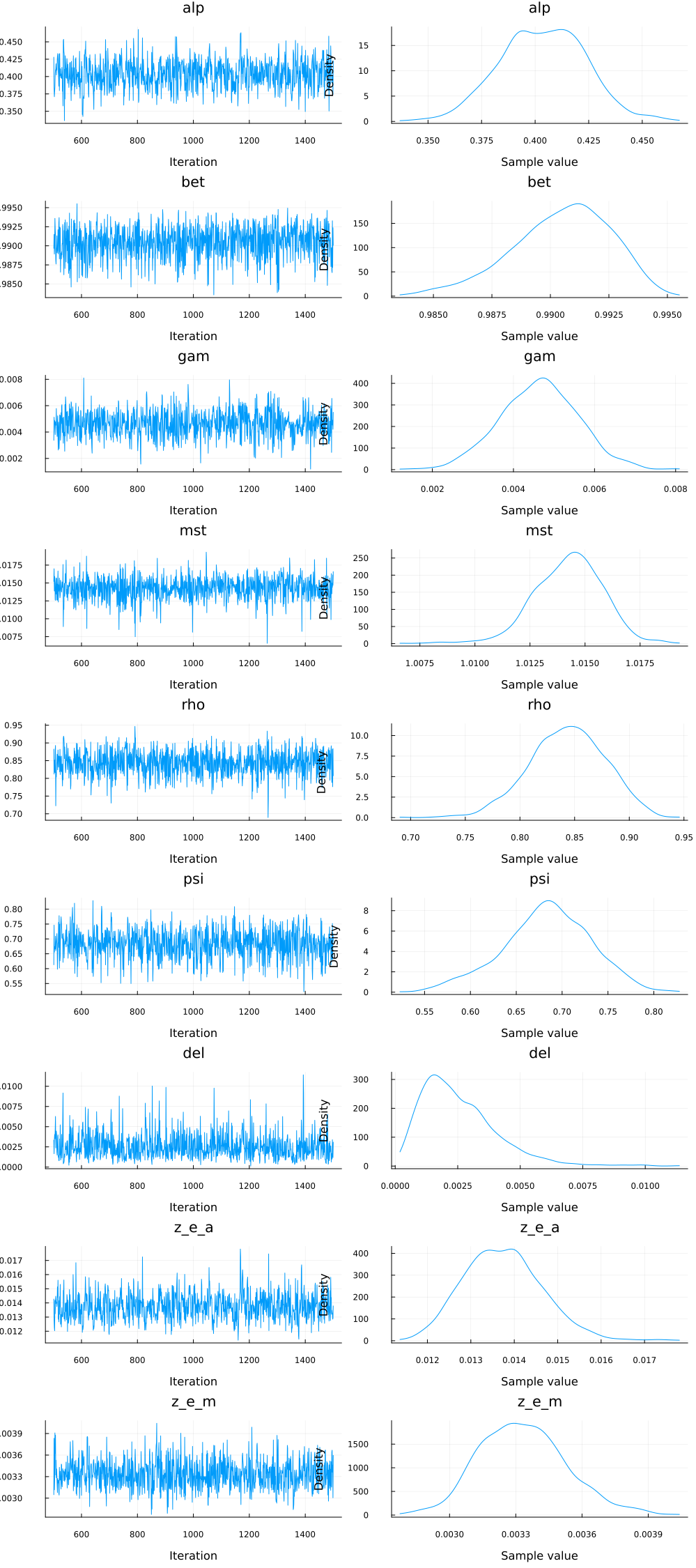
In order to understand the posterior distribution and the sequence of samples they are plotted:
julia> using StatsPlotsjulia> plot(chain_NUTS);
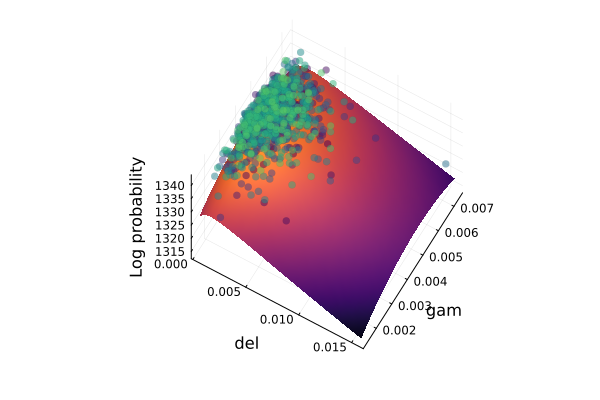
Next, the posterior loglikelihood is plotted along two parameters dimensions, with the other parameters kept at the posterior mean, and the samples are added to the visualisation. This visualisation allows understanding the curvature of the posterior and puts the samples in context.
julia> import DynamicPPL: logjointjulia> parameter_mean = collect(values(Turing.mean(chain_NUTS); parameters_only = true))9-element Vector{Float64}: 0.40506911567682 0.9905552981330771 0.004623149525277305 1.0142505682233989 0.8453997241937198 0.6853893964021719 0.002485013924988703 0.013768561750630421 0.003326929238435069julia> pars = (; parameters = parameter_mean);julia> logjoint(FS2000_loglikelihood, pars)1343.4230854031944julia> function calculate_log_probability(par1, par2, pars_idx, base_pars, model) pvec = copy(base_pars.parameters) pvec[pars_idx[1]] = par1 pvec[pars_idx[2]] = par2 logjoint(model, (; parameters = pvec)) endcalculate_log_probability (generic function with 1 method)julia> granularity = 32;julia> par1 = :del;julia> par2 = :gam;julia> param_syms = Symbol.(get_parameters(FS2000));julia> paridx1 = indexin([par1], param_syms)[1];julia> paridx2 = indexin([par2], param_syms)[1];julia> parameter_samples = chain_NUTS[:parameters, stack = true]┌ 1000×1×9 DimArray{Float64, 3} Parameter(parameters) ┐ ├─────────────────────────────────────────────────────┴──── dims ┐ ↓ iter Sampled{Int64} 501:1500 ForwardOrdered Regular Points, → chain Sampled{Int64} 1:1 ForwardOrdered Regular Points, ↗ AnonDim Sampled{Int64} 1:9 ForwardOrdered Regular Points └────────────────────────────────────────────────────────────────┘ [:, :, 1] ↓ → 1 501 0.402184 502 0.351391 503 0.421388 ⋮ 1497 0.423729 1498 0.435213 1499 0.464052 1500 0.457458julia> par_range1 = collect(range(minimum(parameter_samples[:, :, paridx1]), stop = maximum(parameter_samples[:, :, paridx1]), length = granularity));julia> par_range2 = collect(range(minimum(parameter_samples[:, :, paridx2]), stop = maximum(parameter_samples[:, :, paridx2]), length = granularity));julia> p = surface(par_range1, par_range2, (x,y) -> calculate_log_probability(x, y, [paridx1, paridx2], pars, FS2000_loglikelihood), camera=(30, 65), colorbar=false, color=:inferno);julia> joint_loglikelihood = vec(collect(logjoint(FS2000_loglikelihood, chain_NUTS)));julia> scatter3d!(vec(collect(parameter_samples[:, :, paridx1])), vec(collect(parameter_samples[:, :, paridx2])), joint_loglikelihood, mc = :viridis, marker_z = collect(1:length(joint_loglikelihood)), msw = 0, legend = false, colorbar = false, xlabel = string(par1), ylabel = string(par2), zlabel = "Log probability", alpha = 0.5);julia> pPlot{Plots.GRBackend() n=2}
Find posterior mode
Other than the mean and median of the posterior distribution the mode can also be calculated as follows:
julia> modeFS2000 = Turing.maximum_a_posteriori(FS2000_loglikelihood,
                                               adtype = AutoMooncake(; config=nothing),
                                               initial_params = Turing.InitFromParams((; parameters = FS2000.parameter_values)))ModeResult
  ├ estimator    : Turing.Optimisation.MAP
  ├ lp           : 1343.7491257506185
  ├ params       : VarNamedTuple with 1 entry
  │                └ parameters => [0.4027213061413159, 0.9909439049258357, 0.004550077284871631, 1.014322732114242, 0.8457080502069314, 0.6910342545074338, 0.001635313240222382, 0.01347992249531296, 0.0032575451181054696]
  │ linked       : true
  └ (2 more fields: optim_result, ldf)
Model estimates given the data and the model solution
Having found the parameters at the posterior mode model estimates of the shocks which explain the data used to estimate it can be retrieved. This can be done with the get_estimated_shocks function:
julia> get_estimated_shocks(FS2000, data, parameters = NamedTuple(modeFS2000.params).parameters)2-dimensional KeyedArray(NamedDimsArray(...)) with keys:
↓   Shocks ∈ 2-element Vector{Symbol}
→   Periods ∈ 192-element UnitRange{Int64}
And data, 2×192 Matrix{Float64}:
             (1)         (2)         …  (191)         (192)
  (:e_a₍ₓ₎)    3.07802     2.02956          0.31192       0.0219214
  (:e_m₍ₓ₎)   -0.338786    0.529109        -0.455173     -0.596633
As the first argument the model is passed, followed by the data (in levels), and then the parameters at the posterior mode. The model is solved with this parameterisation and the shocks are calculated using the Kalman smoother.
The model was estimated on two variables but the model allows examining all variables given the data. Looking at the estimated variables can be done using the get_estimated_variables function:
julia> get_estimated_variables(FS2000, data)2-dimensional KeyedArray(NamedDimsArray(...)) with keys:
↓   Variables ∈ 18-element Vector{Symbol}
→   Periods ∈ 192-element UnitRange{Int64}
And data, 18×192 Matrix{Float64}:
                 (1)          (2)          …  (191)           (192)
  (:P)             0.585869     0.596628          0.560845        0.559733
  (:Pᴸ⁽¹⁾)         0.585108     0.595478          0.561547        0.560631
  (:R)             1.02576      1.02692           1.01966         1.01858
  (:W)             2.99871      3.01049           2.96335         2.9599
  (:c)             1.73321      1.7013     …      1.80033         1.80164
  (:cᴸ⁽¹⁾)         1.73494      1.7039            1.79936         1.80039
   ⋮                                       ⋱      ⋮
  (:k)            53.4886      52.032            56.2707         56.2515
  (:l)             0.724385     0.733136          0.705017        0.704388
  (:log_gp_obs)   -0.0044494    0.0038943         0.00295712      0.00285919
  (:log_gy_obs)    0.0376443    0.026348   …      0.00793817      0.00487735
  (:m)             1.01686      1.01822           1.00971         1.00845
  (:n)             0.241598     0.243599          0.237911        0.237975
  (:y)             2.1224       2.11046           2.14601         2.14608
Since the model was already solved with the parameters at the posterior mode there is no need to do so again. The function returns a KeyedArray (from the AxisKeys package) with the values of the variables in levels at each point in time.
Another useful tool is a historical shock decomposition. It allows understanding the contribution of the shocks for each variable. This can be done using the get_shock_decomposition function:
julia> get_shock_decomposition(FS2000, data)3-dimensional KeyedArray(NamedDimsArray(...)) with keys:
↓   Variables ∈ 18-element Vector{Symbol}
→   Shocks ∈ 3-element Vector{Symbol}
◪   Periods ∈ 192-element UnitRange{Int64}
And data, 18×3×192 Array{Float64, 3}:
[showing 3 of 192 slices]
[:, :, 1] ~ (:, :, 1):
                 (:e_a₍ₓ₎)     (:e_m₍ₓ₎)     (:Initial_values)
  (:P)            0.0148888    -0.00108998    0.00810035
  (:Pᴸ⁽¹⁾)        0.0146127    -0.000913525   0.00743931
  (:R)           -6.78119e-16  -0.000955353   0.0031234
   ⋮
  (:log_gy_obs)   0.0328867     8.71844e-5    0.000120402
  (:m)           -0.0          -0.00111942    0.00365979
  (:n)            0.00322234    3.46638e-5    0.000868554
  (:y)           -0.018474      0.000187179  -0.0062412

[:, :, 97] ~ (:, :, 97):
                 (:e_a₍ₓ₎)     (:e_m₍ₓ₎)     (:Initial_values)
  (:P)            0.0288478     0.00602704    0.000719126
  (:Pᴸ⁽¹⁾)        0.0283128     0.00503281    0.000705791
  (:R)           -7.66178e-15   0.00539571    3.21953e-10
   ⋮
  (:log_gy_obs)  -0.0168618     0.000336676   7.85288e-6
  (:m)           -3.6279e-16    0.00632233    3.77243e-10
  (:n)            0.00624343   -0.000223709   0.000155638
  (:y)           -0.0357943    -0.000897025  -0.000892291

[:, :, 192] ~ (:, :, 192):
                 (:e_a₍ₓ₎)     (:e_m₍ₓ₎)     (:Initial_values)
  (:P)            0.00129293   -0.00565097    0.000121485
  (:Pᴸ⁽¹⁾)        0.00126895   -0.00472692    0.000119232
  (:R)           -2.15194e-16  -0.00500928    1.12757e-17
   ⋮
  (:log_gy_obs)   0.000247177   7.87663e-5    1.32661e-6
  (:m)            4.58977e-17  -0.00586953    4.25007e-17
  (:n)            0.000279824   0.000195656   2.62925e-5
  (:y)           -0.00160426    0.000901756  -0.000150738
A 3-dimensional array is returned with variables, shocks, and time periods as dimensions. The shocks dimension also includes the initial value as a residual between the actual value and what was explained by the shocks. This computation also relies on the Kalman smoother.
Last but not least, the model estimates and the shock decomposition can also be plotted. The model estimates plot, using plot_model_estimates:
julia> plot_model_estimates(FS2000, data)4-element Vector{Any}:
 Plot{Plots.GRBackend() n=42}
 Plot{Plots.GRBackend() n=42}
 Plot{Plots.GRBackend() n=44}
 Plot{Plots.GRBackend() n=10}
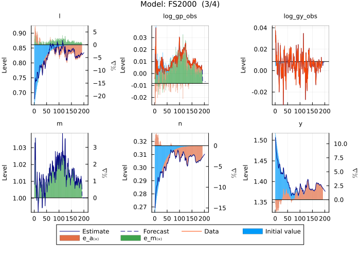
shows the variables of the model (blue), data (red), the shock decomposition for each endogenous variable and in the last panel the estimated shocks used to estimate the model.